
A topographic map is a detailed and accurate two-dimensional representation of natural and human-made features on the Earth's surface. These maps are used for many applications, from camping, hunting, fishing, and hiking to urban planning, resource management, and surveying. The most distinctive characteristic of a topographic map is that the three-dimensional shape of the Earth's surface is modeled with contour lines. Contours are imaginary lines that connect locations of similar elevation. Contours make it possible to represent mountain height and slope steepness on a two-dimensional map surface. Topographic maps also use various symbols to describe natural and human-made features such as roads, buildings, quarries, lakes, streams, and vegetation.
Topographic maps have been made by the United States Geological Survey (USGS) since 1879 (Figure 2.22). Coverage of the United States is available at scales of 1:20,000 (Puerto Rico only), 1:24,000, 1:25,000 (metric), 1:30,000 (Puerto Rico only), 1:62,250, 1:63,360 (Alaska only), 1:100,000, and 1:250,000. Canadian topographic maps produced by the National Topographic System of Canada (NTS) are generally available in two scales: 1:50,000 and 1:250,000. Topographic maps at a scale of 1:25,000 are relatively large-scale, and a typical map sheet covers an area of approximately 125 to 165 km2. At this scale, features as small as a single home can be easily shown (Figure 2.23). The smaller-scale 1:250,000 topographic map is more suitable for general reconnaissance purposes (Figure 2.24). A map of this scale covers the same area of land as sixty-four 1:25,000 scale maps.
Topographic Map Symbols
Topographic maps use a variety of symbols to represent natural and human-constructed features found in the environment. The symbols used to describe features can be of three types: points, lines, and polygons. Points are used to depict features like bridges and buildings. Lines are used to graphically illustrate linear features, such as roads, railways, and rivers. Polygons are used to characterize features such as buildings, water bodies, and areas of specific land use. Some polygons are identified only by color. For example, urban land use is often shaded pink, natural vegetation is green, glaciers are pale blue, and cropland is white.
The symbols used on topographic maps have been standardized to simplify map construction. Standardization also makes using topographic maps easier because the map user needs to learn only one system of symbolization. A description of some of the symbols used is shown in Figure 2.25. Despite standardization, we can sometimes find topographic maps that use different symbols to depict the same feature. This problem occurs because the symbols used in these maps are continuously refined over time.
Contour Lines
Topographic maps can describe vertical information with contour lines (contours). A contour line is an isoline that connects points on a map with the same elevation. Contours are often drawn on a map at a uniform vertical distance. This distance is called the contour interval. The map in Figure 2.26 shows contour lines with a 100-meter (m) interval. Note that every fifth brown contour line is bolded and labeled with the appropriate elevation. These contours are called index contours. Figure 2.26 shows index contours for heights of 100, 200, 300, 400 m, etc. The interval at which contours are drawn on a map depends on the amount of relief depicted and the map's scale.
Contour lines provide a simple, effective way to describe landscape configuration on a two-dimensional map. The arrangement, spacing, and shape of the contours give the map user some idea of the actual topographic configuration of the land surface. Contour intervals that are spaced closely together describe a steep slope. Widely spaced contours indicate gentle slopes. Contour lines that V upwards indicate the presence of a stream valley. Ridges are shown by contours that V downwards.
Topographic Map Profiles
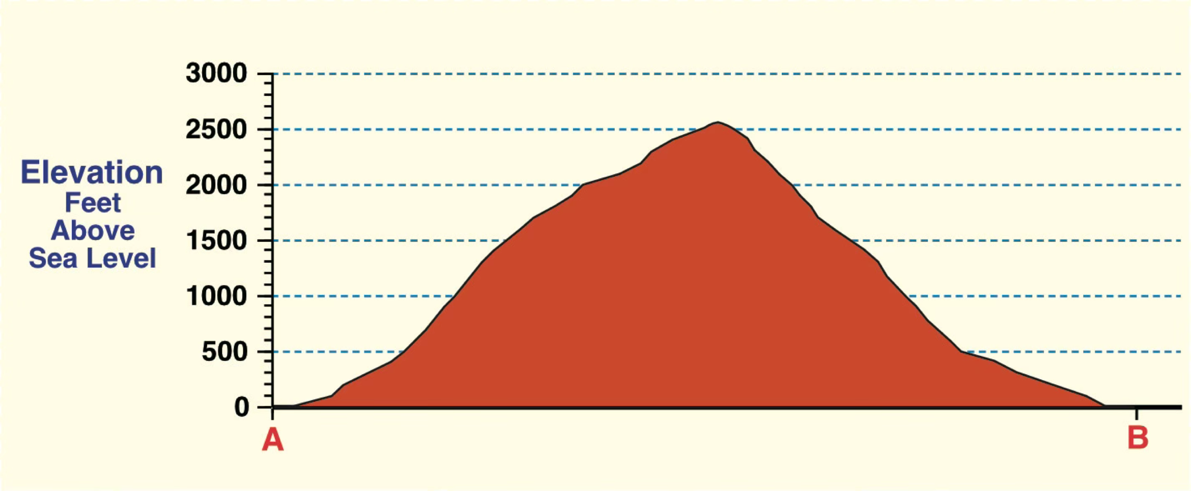
A topographic profile is a two-dimensional diagram that describes the landscape in a vertical cross-section. Topographic profiles are often created from the contour information found on topographic maps. The simplest way to construct a topographic profile is to place a sheet of blank paper along a horizontal transect of interest. From the map, the elevations of the various contours are transferred onto the edge of the paper. On a sheet of graph paper, we use the X-axis to represent the horizontal distance covered by a transect. The Y-axis represents the vertical dimension and measures changes in map elevation. Most people exaggerate the scale of elevation on the Y-axis to make changes in relief stand out. The next step in this process is to place the beginning of the transect, as transcribed on the piece of paper, at the intersection of the X and Y axes on the graph paper. The contour information from the paper's edge is then carefully copied onto the graph paper. Figure 2.27 describes a topographic profile drawn from the information found on the transect A - B in Figure 2.26.
Measuring Distance on Topographic Maps
On a previous webpage, we learned that depicting Earth's three-dimensional surface on a two-dimensional map creates several distortions in distance, area, and direction. It is possible to make somewhat equidistant maps. However, even these types of maps have some form of distance distortion. Equidistance maps can only control distortion along either latitude or longitude lines. Distance is often correct on equidistance maps only along the direction of latitude.
Distance distortion is usually insignificant at large scales, such as 1:125,000 or larger. An example of a large-scale map is a standard topographic map. On large-scale maps, measuring straight-line distance is simple. Distance is first measured on the map using a ruler. This measurement is then converted to an actual-world distance using the map's scale. For example, if we measured a distance of 10 cm on a map that had a scale of 1:10,000, we would multiply 10 (distance) by 10,000 (scale). Thus, the actual distance in the real world would be 100,000 cm.
Measuring distance along map features that are not straight is a little more complicated. One technique that can be employed for this task is to use several straight-line segments. The accuracy of this method is dependent on the number of line segments used (Figure 2.28). Another technique for measuring curvilinear map distances is to use a mechanical device called an opisometer (Figure 2.29). This device uses a small rotating wheel that records the distance traveled.
Measuring Direction on Topographic Maps
Like distance, direction is difficult to measure on maps because of the distortion that projection systems produce. However, this distortion is relatively small on maps with scales larger than 1:125,000. Direction is usually measured relative to the location of the North or South Pole. Directions determined from these locations are said to be relative toTrue NorthorTrue South. The magnetic poles can also be used to measure direction. However, these points on Earth are located at different spatial positions from the geographic North and South Poles. The North Magnetic Pole is located at 86° 39’ North, 162° 52’ East in the middle or the Arctic Ocean. In the Southern Hemisphere, the South Magnetic Pole is located in Commonwealth Day, Antarctica, and has a geographical location of 63° 48’ South, 134° 54’ East. The magnetic poles are also not fixed and shift their spatial position over time.
Topographic maps usually include a declination diagram (Figure 2.30). In Northern Hemisphere maps, declination diagrams describe the angular difference between Magnetic North and True North. On the map, the angle of True North is parallel to the depicted lines of longitude. Declination diagrams also show the direction of Grid North. Grid North is an angle parallel to the easting lines found on the Universal Transverse Mercator (UTM) grid system.
In the field, the direction of features is often determined by a magnetic compass that measures angles relative to Magnetic North. Using the declination diagram on a map, individuals can convert their field-measured magnetic directions to directions relative to Grid or True North. Compass and map directions can be described using either the azimuth or bearing systems. The azimuth system calculates direction in degrees of a full circle. A full circle has 360 (Figure 2.31). In the azimuth system, north points in either the 0° or 360° direction. East and west have an azimuth of 90° and 270°, respectively. Due south has an azimuth of 180°.
The bearing system divides the direction into four quadrants of 90° each. In this system, north and south are the dominant directions. Measurements are determined in degrees from one of these directions to either east or west. The measurement of two angles based on this system is described in Figure 2.32.


FIGURE 2.27 The following topographic profile shows the vertical change in surface elevation along the transect A - B from Figure 2.26. A vertical exaggeration of about 4.2× was used in the profile (horizontal scale = 1:50,000; vertical scale = 1:12,000; vertical exaggeration = vertical scale/horizontal scale). Image Copyright: Michael Pidwirny.
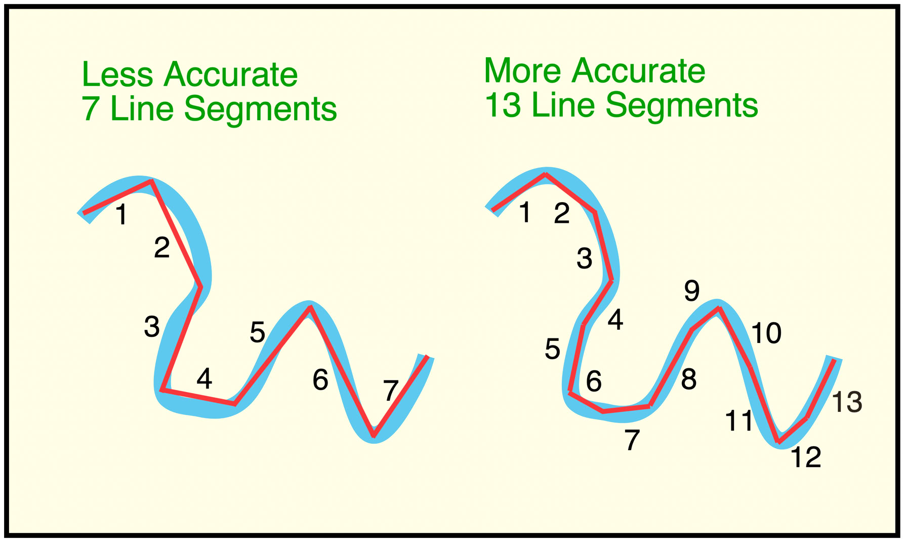
FIGURE 2.28 Measurement of distance on a map feature using straight-line segments. Accuracy increases with the number of segments used. Image Copyright: Michael Pidwirny.

FIGURE 2.29 An opisometer is a mechanical instrument used to measure distance on maps. Image Copyright: Michael Pidwirny.


FIGURE 2.31 The Azimuth system for measuring direction is based on the 360 degrees in a full circle. The illustration shows the angles associated with the major cardinal points of the compass. Note that angles are determined clockwise from north. Image Copyright: Michael Pidwirny.
FIGURE 2.22 Part of the 1:24,000 United States Geological Survey topographic map of Santa Barbara, California. This map shows that many different symbols are used to display natural and human-made features in this landscape. Color shading is used to categorize land use. Pink indicates the urban built area, blue shows the ocean and other water bodies, light purple depicts extensions of urban areas, and green defines areas of natural vegetation. Image Source: United States Geological Survey - Topographic Maps.
FIGURE 2.23 Top three-quarters of the 1:24,000 United States Geological Survey topographic map for Sieler, Washington. Note that at this scale, houses and other buildings are clearly illustrated. Image Source: United States Geological Survey - Topographic Maps.
FIGURE 2.24 Part of the 1:250,000 United States Geological Survey topographic map of Jackson, Mississippi, and Louisiana. Note that some urban settlements appear at this scale as a single point on the map. Image Source: United States Geological Survey - Topographic Maps.
FIGURE 2.25 Some of the symbols used in United States Geological Survey topographic maps. Image Source: United States Geological Survey - Topographic Maps.
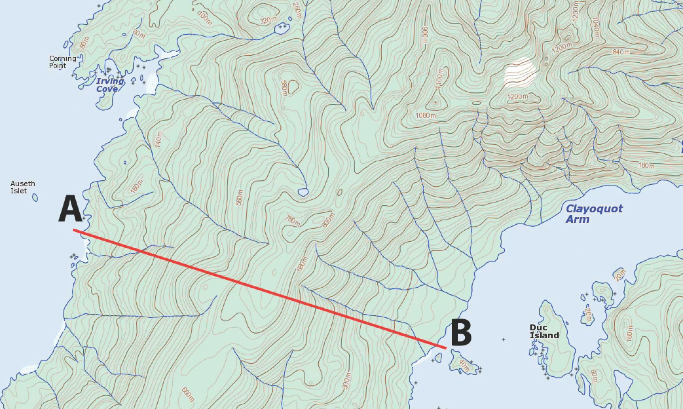
FIGURE 2.26 A topographic map with contour lines. Portion of the Tofino 1:50,000 National Topographic System of Canada map sheet 092F4. The brown lines drawn on this map are contour lines. Each line represents a 25-meter (m) increase in elevation. The bold brown contour lines are called index contours. The index contours are labeled with their corresponding elevations, which increase by 100 meters (m). Note that the blue line drawn to separate water from land represents an elevation of 0 meters or sea level. Modified Image Source: Natural Resources Canada - Toporama.
FIGURE 2.30 This declination diagram describes the angular difference between Grid, True, and Magnetic North. The declination diagram shows the angular differences between Grid North and True North, and between Grid North and Magnetic North. Angles on maps are usually measured relative to Grid North. Using the declination diagram, one can convert the Grid angle or azimuth into True or Magnetic equivalents. Image Copyright: Michael Pidwirny.

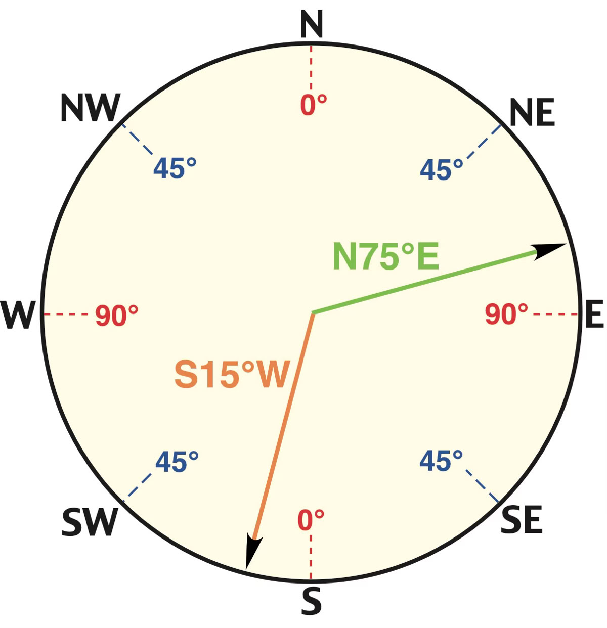
FIGURE 2.32 The bearing system uses four quadrants of 90° to measure direction. The illustration shows two direction measurements. These measurements are made relative to either north or south. North and south are given the measurement of 0°. East and west both have a value of 90°. The first measurement (green) is found in the north - east quadrant. As a result, its measurement is north 75° to the east or N75°E. The first measurement (orange) is found in the south - west quadrant. Its measurement is south 15° to the west or S15°W. Image Copyright: Michael Pidwirny.